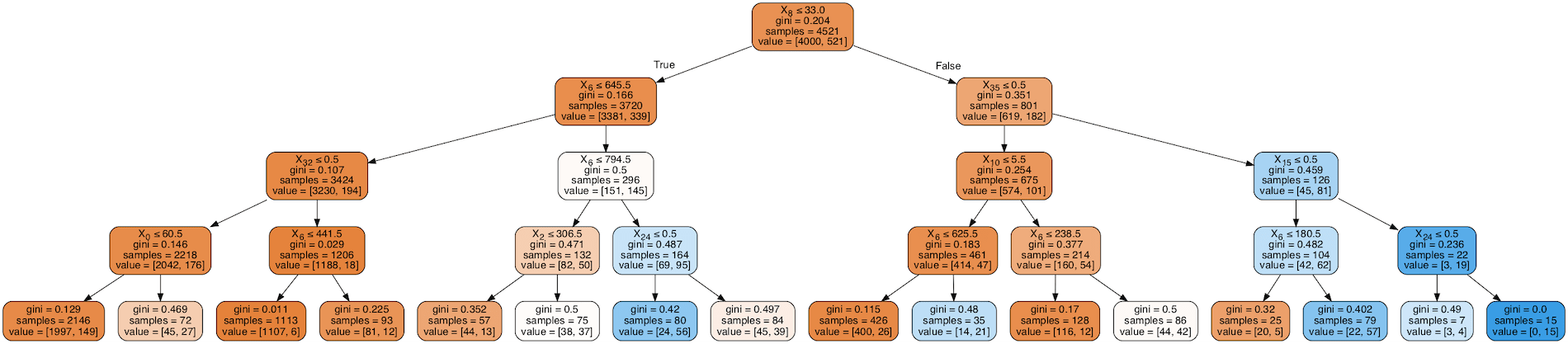
In this post we are going to manage a Classification problem, by using some CART models (Classification And Regression Trees).
We will use the following Bank Marketing Data Set dataset, provided by the UCI Machine Learning Repository:
ref. [Moro et al., 2014] S. Moro, P. Cortez and P. Rita. A Data-Driven Approach to Predict the Success of Bank Telemarketing. Decision Support Systems, Elsevier, 62:22-31, June 2014
These are the results about some direct marketing campaigns carried out by a Portuguese bank by using outbound contact center calls, to try to sell repo financial products to customers.
The labeled output data we are interested in predicting are “binary” (column y): “yes” in the event that customers have accepted the bank deposit offer or “no” if the offer has been rejected.
Let’s import some useful libraries with scikit-learn:
import pandas as pd
from sklearn import ensemble
from sklearn.metrics import mean_absolute_error
import matplotlib.pyplot as plt
import matplotlib.ticker as ticker
import matplotlib.animation as animation
import numpy as np
from sklearn import preprocessing
from sklearn.preprocessing import LabelEncoder
from sklearn.preprocessing import OneHotEncoder
from sklearn.ensemble import RandomForestClassifier
from sklearn.tree import DecisionTreeClassifier
from sklearn.datasets import make_classification
import seaborn as sns; sns.set()
from sklearn.model_selection import train_test_split
from sklearn.metrics import classification_report
Let’s import our dataset thus to have it available inside a dataframe we can easily manipulate.
df = pd.read_csv(‘http://gosmar.eu/ml/bank.csv’)
print(“Lenght:”, len(df))
print(df.info())
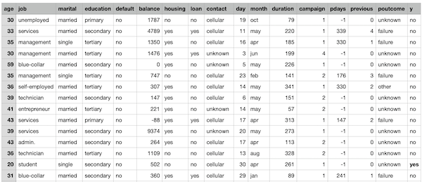
Let’s take a look at these data:
Lenght: 4521
<class 'pandas.core.frame.DataFrame'>
RangeIndex: 4521 entries, 0 to 4520
Data columns (total 17 columns):
age          4521 non-null int64
job          4521 non-null object
marital      4521 non-null object
education    4521 non-null object
default      4521 non-null object
balance      4521 non-null int64
housing      4521 non-null object
loan         4521 non-null object
contact      4521 non-null object
day          4521 non-null int64
month        4521 non-null object
duration     4521 non-null int64
campaign     4521 non-null int64
pdays        4521 non-null int64
previous     4521 non-null int64
poutcome     4521 non-null object
y            4521 non-null object
We can see 4521 observations from customers contacted by the contact center to offer the banking deposit.
As you can see we know the age, job, marital status, and other information about each potential customer.
The campaign feature, in particular, contains the number of calls the contact center has tried to make to each potential customer. If we sum-up the values of this column, we get the number of total calls made: 12.630.
Let’s see how many of these 4521 customers have purchased the financial product:
len(df[df[“y”] == ‘yes’])
result: 521
Now, let’s suppose we are able to predict whether a potential customer will buy this banking product or not, based on the training data available to us… Can you see how many of the 12,630 calls – and the amount of the customer care agent time – would we have saved?
Also, how many potential customers could this call center avoid to call useless?
Let’s analyze the feature correlation:
fig, ax = plt.subplots(figsize=(14,10))
ax = sns.heatmap(df.corr(), cmap=”YlGnBu”, annot = True)
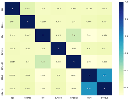
Apart from a couple of features, the others are not very correlated to each other. This reduces the risk of overfitting for our CART-based model .
Let’s further analyze data type: we can note there are a lot of non-numerical features. This situation needs to be fixed if we want to be able to use our machine learning algorithm.
As a result we are going to use some machine learning encoding techniques in order to transform our entire dataset into numerical values.
le = LabelEncoder()
le.fit(df[‘default’])
df[‘default’] = le.transform(df[‘default’])
le.fit(df[‘housing’])
df[‘housing’] = le.transform(df[‘housing’])
le.fit(df[‘loan’])
df[‘loan’] = le.transform(df[‘loan’])
le.fit(df[‘y’])
df[‘y’] = le.transform(df[‘y’])
mapper = dict({‘jan’:1,’feb’:2,’mar’:3,’apr’:4,’may’:5,’jun’:6,’jul’:7,’aug’:8,’sep’:9,’oct’:10,’nov’:11,’dec’:12})
df[‘month_new’] = df[‘month’].map(mapper)
df.drop([“month”], axis = 1, inplace = True)
df=pd.get_dummies(df,columns=[‘job’,’marital’,’education’,’contact’,’poutcome’])
print(len(df.columns))
result: 38
We have transformed our dataset from 17 mixed features to 38 purely numeric features.
We are now ready for the actual training phase.
Let’s separate the independent variables from the labeled feature (y):
X=df.drop(‘y’,axis=1)
y=df[‘y’]
We are going to use 70% of our dataset for the training phase and 30% for the test phase:
X_train,X_test,y_train,y_test=train_test_split(X,y,test_size=0.3,shuffle=True)
We can now move forward with the Random Forest model and fitting it.
model = ensemble.RandomForestClassifier(n_estimators=200, criterion=’gini’, max_depth=None,
min_samples_split=2, min_samples_leaf=1, min_weight_fraction_leaf=0.0,
max_features=’auto’, max_leaf_nodes=None, min_impurity_decrease=0.0,
min_impurity_split=None, bootstrap=True, oob_score=False, n_jobs=None,
random_state=None, verbose=0, warm_start=False,
class_weight={0:1,1:2})
model.fit(X_train,y_train)
As you can see, we have used 200 estimators (200 random trees) and we have performed a stratified sampling technique to give more weight to the class y = 1 (which is much less present inside our date, but important).
This should improve the performance of our model, by reducing the associated Bias.
Let’s now move to the accuracy evaluation and the confusion matrix visualization:
print(“Accuracy on training set is : {}”.format(model.score(X_train, y_train)))
print(“Accuracy on test set is : {}”.format(model.score(X_test, y_test)))
y_test_pred = model.predict(X_test)
print(classification_report(y_test, y_test_pred))
Accuracy on training set is : 1.0
Accuracy on test set is : 0.9086219602063376
              precision    recall  f1-score   support

           0       0.92      0.99      0.95      1214
           1       0.70      0.23      0.35       143

    accuracy                           0.91      1357
   macro avg       0.81      0.61      0.65      1357
weighted avg       0.89      0.91      0.89      1357
#Print the confusion matrix
from sklearn import metrics
print(metrics.confusion_matrix(y_test, y_test_pred))
[[1200   14]
 [ 110   33]]
The accuracy value of 0.91 can also be obtained from the ratio between the sum of the diagonal values and the total values inside the confusion matrix.
Well, we got 91% accuracy … Not bad for a CART-based classifier!
We can also conclude that – if the Portuguese bank in question had used these machine learning techniques before carrying out its marketing campaign – it would probably have been able to make only about 1500 calls* to reach the same conversion rate (instead of over 12,000) with a 9% error margin!
*Il ragionamento tiene conto già del fatto che i 521 clienti che hanno accettato l’offerta fossero stati chiamati in media circa 3 volte cadauno.
Interested in learning more about Machine Learning and AI applications?
Here you can find a book about it:
https://www.amazon.com/dp/B08GFL6NVM