In this first post we will play a bit with Linear Regression in order to get confidence with some key concepts about machine learning.
Deep Learning Convolutional Neural Network, Recurring Neural Network, Support Vector Machine, Logistic Regression are great techniques for complex prediction, even the non-linear ones.
However Linear Regression is a great way to start when you have to perform prediction about data generally linearly correlated data.

Let’s consider the Australian athletes data set: a nice dataset collected in a study of how data on various characteristics of the blood varied with sport body size and sex of the athlete. These data were the basis for the analyses reported in Telford and Cunningham (1991).
Anybody interested in knowing more about that study can reference to the Telford, R.D. and Cunningham, R.B. 1991. Sex, sport and body-size dependency of hematology in highly trained athletes. Medicine and Science in Sports and Exercise 23: 788-794: https://europepmc.org/article/med/1921671
We are going to use Pyhton with Jupyter Notebook for such a model.
Let’s import some useful libraries to start:
from sklearn.metrics import classification_report
from sklearn import metrics
import pandas as pd
import statsmodels.api as sm
import numpy as np
import matplotlib.pyplot as plt
%matplotlib inline
Here we are going to import the dataset:
#Import dataset inside the dataframe df
df = pd.read_csv(‘http://gosmar.eu/ml/ais.csv’, index_col=0)
print(df.head(2))
print(“Lenght:”, len(df_male))
Let’s have a look at the features (columns) inside it:
  rcc  wcc  hc  hg  ferr  bmi  ssf  pcBfat  lbm  ht  wt  sex  sport
1 3.96 7.5 37.5 12.3 60 20.56 109.1 19.75 63.32 195.9 78.9 f B_Ball
2 4.41 8.3 38.2 12.7 68 20.67 102.8 21.30 58.55 189.7 74.4 f B_Ball

Lenght: 102
We would like to keep it simply by selecting only two features: the first will be our independent variable, the second the target label to predict. We are looking for two features with some correlation between them.
A good way to evaluate the correlation between features is to print the heatmap!
import seaborn as sns; sns.set()
fig, ax = plt.subplots(figsize=(14,10))
ax = sns.heatmap(df.corr(), cmap=”YlGnBu”, annot = True)
Here we are with the result:
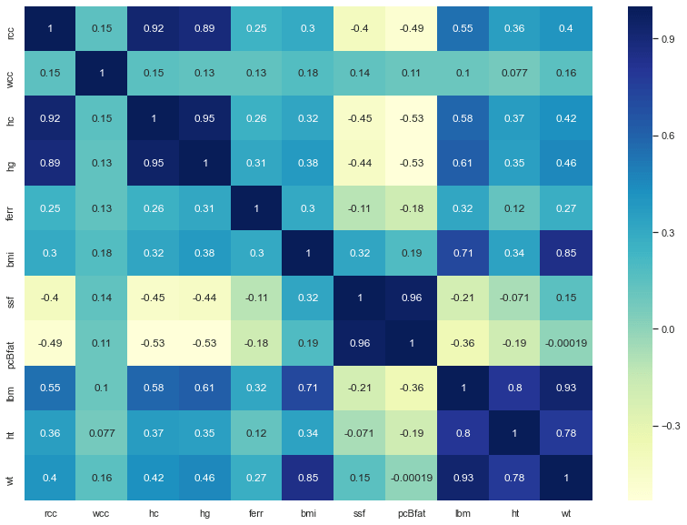
The darker is the colour, the more the features are correlated, so we are going to select:
X (independent feature) = bmi
Y (target feature) = lbm
Where bmi is the Body Mass Index, kg and lbm is the Lean Body Mass, kg.
Two blood parameters pretty much useful for athletes.
Let’s do some dimensionality reduction in order to drop a lot of features we will not use for sure:
df_new=df.drop(['rcc','hc','hg','ferr','ssf','pcBfat','sport'], axis=1)
print(df_new.head(6))
print(len(df_new))
result:
 wcc    bmi    lbm     ht    wt sex
1  7.5  20.56  63.32  195.9  78.9   f
2  8.3  20.67  58.55  189.7  74.4   f
3  5.0  21.86  55.36  177.8  69.1   f
4  5.3  21.88  57.18  185.0  74.9   f
5  6.8  18.96  53.20  184.6  64.6   f
6  4.4  21.04  53.77  174.0  63.7   f
202
Let’s now split our dataset in two different dataframes: the first one with the male data and the second one with the female data:

df_male = df_new.loc[df_new.sex == ‘m’]
print(df_male.head(2))
print(“Lenght:”, len(df_male))
result:
wcc    bmi   lbm     ht    wt sex
101  7.1  22.46  61.0  172.7  67.0   m
102  7.6  23.88  69.0  176.5  74.4   m
Lenght: 102

df_female = df_new.loc[df_new.sex == ‘f’]
print(df_female.head(2))
print(“Lenght:”, len(df_female))
result:
wcc    bmi    lbm     ht    wt sex
1  7.5  20.56  63.32  195.9  78.9   f
2  8.3  20.67  58.55  189.7  74.4   f
Lenght: 100
We can now setup the independent variable (bmi) and the target value (lbm) for the training phase:
#To_be_predicted
y1_male = df_male[‘lbm’]
#Intependent vars
X1_male = df_male[‘bmi’]
#Add constant to better fit the linear model
X1_male = sm.add_constant(X1_male.to_numpy())
We are going to use the statsmodels.regression.linear_model.OLS class as our linear regression model:
model = sm.OLS(y1_male, X1_male)
It’s now time to fit our model. The fitting procedure is the phase where we adapt the model to the training dataset and we are going to build the learned function
model = model.fit()
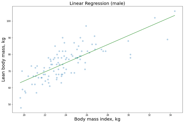
Now we want to display the training data or lmi as a function of the bmi that we recover from our imported dataset and the linear regression function related to the model just built. In this case it will be a straight line Y = c1 + c2X.
Let’s use some visualization options to do it:
#Create the X array from the min to the max observations
X_obs = np.linspace(X1_male[:,1].min(), X1_male[:,1].max(), len(df_male))[:, np.newaxis]
X_obs = sm.add_constant(X_obs)
#Let’s calculate the predicted values
y_pred = model.predict(X_obs)
fig = plt.figure()
fig.subplots_adjust(top=3.8, right = 1.9)
ax1 = fig.add_subplot(211)
plt.scatter(X1_male[:,1], y1_male, alpha=0.3) # Plot the raw data
plt.title(“Linear Regression (male)”, fontsize=20)
plt.xlabel(“Body mass index, kg”, fontsize=20)
plt.ylabel(“Lean body mass, kg”, fontsize=20)
plt.plot(X_obs[:, 1], y_pred, ‘g’, alpha=0.9) # Add the regression line, colored in red
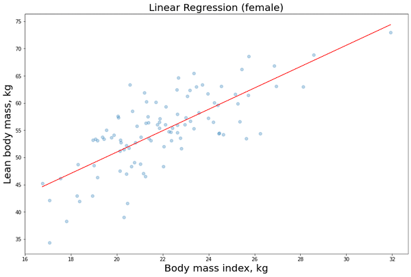
We just need to repeat the same procedure for the female data:
#To_be_predicted
y1_female = df_female[‘lbm’]
#Intependent vars
X1_female = df_female[‘bmi’]
#Add constant to better fit the linear model
X1_female = sm.add_constant(X1_female.to_numpy())
model = sm.OLS(y1_female, X1_female)
model = model.fit()
#Create the X array from the min to the max observations
X_obs = np.linspace(X1_female[:,1].min(), X1_female[:,1].max(), len(df_female))[:, np.newaxis]
X_obs = sm.add_constant(X_obs)
#Let’s calculate the predicted values
y_pred = model.predict(X_obs)
fig = plt.figure()
fig.subplots_adjust(top=3.8, right = 1.9)
ax1 = fig.add_subplot(211)
plt.scatter(X1_female[:,1], y1_female, alpha=0.3) # Plot the raw data
plt.title(“Linear Regression (female)”, fontsize=20)
plt.xlabel(“Body mass index, kg”, fontsize=20)
plt.ylabel(“Lean body mass, kg”, fontsize=20)
plt.plot(X_obs[:, 1], y_pred, ‘r’, alpha=0.9) # Add the regression line, colored in red
Now that we have build our model (training phase), we would like to evaluate some results in order to see if we need to change something on the algorithm and hyperparameters (validation phase):
model.summary()
| Dep. Variable: | lbm | R-squared: | 0.559 |
|---|---|---|---|
| Model: | OLS | Adj. R-squared: | 0.554 |
| Method: | Least Squares | F-statistic: | 124.1 |
| Date: | Sun, 10 May 2020 | Prob (F-statistic): | 4.15e-19 |
| Time: | 19:24:20 | Log-Likelihood: | -293.96 |
| No. Observations: | 100 | AIC: | 591.9 |
| Df Residuals: | 98 | BIC: | 597.1 |
| Df Model: | 1 | ||
| Covariance Type: | nonrobust |
| coef | std err | t | P>|t| | [0.025 | 0.975] | |
|---|---|---|---|---|---|---|
| const | 11.7975 | 3.896 | 3.028 | 0.003 | 4.065 | 19.530 |
| x1 | 1.9599 | 0.176 | 11.140 | 0.000 | 1.611 | 2.309 |
| Omnibus: | 1.486 | Durbin-Watson: | 1.327 |
|---|---|---|---|
| Prob(Omnibus): | 0.476 | Jarque-Bera (JB): | 1.345 |
| Skew: | -0.282 | Prob(JB): | 0.510 |
| Kurtosis: | 2.934 | Cond. No. | 187. |
The values we want to consider for our evaluations are:
- R2 (between zero and one): the closer it is to zero, the less the linear function coefficients c1 and c2 explain the data. The goal is therefore to have R2 as close as possible to one.
- R2 adjusted: it is used if we have multiple independent variables. For example if we had evaluated lmi in function of bmi and other features like ht (height) and wt (total weight). In that case our linear function would have become something like Y = c1 + c2X + c3W + c4Z + …
- Prob (F-statistic): method used to calculate the p-value. The goal is to have this value as low as possible. Low p-value means that our coefficients are reliable for the model, or in statistical jargon the null hypothesis is unlikely.
We told that in this example we are working with a linear model Y = c1 + c2X.
We can easily show c1 and c2:
model.params
result:
const    11.797524
x1        1.959934
…Where c1 = const and c2 = x1
Let’s also show the p-values for each of the previous coefficients:
print(model.pvalues)
const    3.147591e-03
x1       4.150618e-19
In order for the coefficients to be statistically correct, we usually set a threshold of 0.01.
p-values above this threshold means the relative coefficient is not reliable to follow the data variance.
Let’s remind that c1 is the intersection of the straight line with the Y axis, whereas c2 is the slope of the straight line.
In our case we have that c1 is quite reliable and c2 is very reliable!
Wrap-up:
We used a dataset in order to address a regression problem, therefore to predict a value (not a category otherwise we would have faced a classification problem).
First we performed some dataset pre processing (always useful before considering any kind of algorithm): we have identified the features (columns) with more interesting correlation by using the heatmap and we have performed some dimensionality reductions to drop features not useful for our analysis.
After the initial phase, we have performed the training and validation steps where we chose the model and performed the model fit.
Finally we have evaluated the main linear regression parameter results: the linear function coefficients (c1 and c2), the R2 and p-values.
Interested in learning more about Machine Learning and AI applications?
Here you can find a book about it:
https://www.amazon.com/dp/B08GFL6NVM