
Nowadays Machine Learning (ML) techniques are applied in various industries, along with an increasing number of projects and complexity. This generates on one hand the need for greater governance, i.e. the ability to orchestrate and control the development and deploy over the entire ML life cycle (preprocessing, model training, testing, deployment), on the other hand, the need for scalability, i.e. being able to efficiently replicate entire parts of the process, in order to manage multiple ML models.
A recent USA research, carried out to understand the Machine Learning trends for 2021, has conducted a survey on a significant sample of 400 companies: 50% of these are currently managing more than 25 models of ML and 40% of the total runs over 50 ML models. Among large organizations (over 25,000 collaborators) 41% of them turned on to have over 100 ML algorithms in production!
The challenge for these organizations in the years to come will be to manage this growth in order to capitalize on the know-how and to be able to keep control over all these models while reducing the complexity. In other words, being able to manage a significant growth of Machine Learning applications without having to increase the level of complexity by the same order of magnitude.
It is precisely here that MLOps Best Practices take place, literally Machine Learning Operations: tools and procedures aimed at managing the ML life cycle, in order to optimize both the governance and the scalability.
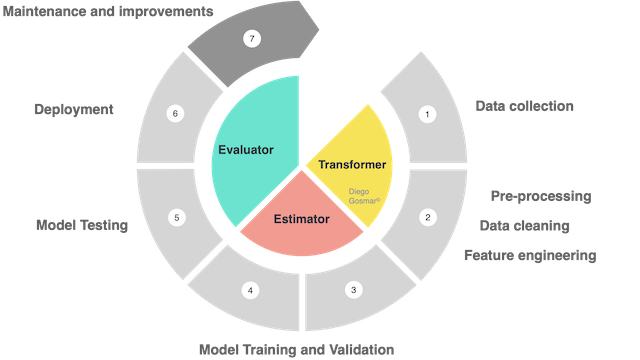
One of the newer ways to control and scale up with ML is to use the pipelines. A full cycle of design, training, testing and deployment – in order to carry out an artificial intelligence application with Machine Learning – typically consists of the following phases: data collection, data cleaning, feature engineering (ie scaling, normalizing, labeling, dimensionality reduction, binning, encoding etc …), Model Training and Validation,
Model Testing, Model deploying, Continuous maintenance and improvement. We also talk about ML life cycle to identify the many different steps involved during these processes.
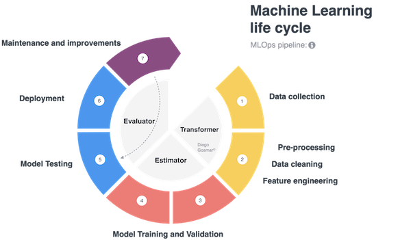
It is interesting to note how many of these steps can be reused in different contexts on multiple AI applications. For example, if we want to test different machine learning algorithms (i.e. 3 different models based on Decision Tree, Deep Learning Neural Network and SVM) on the same dataset, the first steps of data collection, data cleaning, feature engineering will be similar for each of the algorithms that we want to test, while the model training, validation and test phase will change: the ML pipelines address exactly these scenarios making the life cycle modular, governable, repeatable … ultimately scalable!
Let’s now see a practical case of pipelines for MLOps applications by considering a simple example of linear regression and using the PySpark framework available by Databricks.
PySpark is a Python-derived language that inherits the benefits of Apache Spark, designed to perform large-scale dataset pre-processing, analysis and build pipelines for machine learning in order to make the whole process extremely scalable… Moreover it uses a distributed architecture in order to further optimize the scalability.
Thanks to the pipeline concept we will manage a workflow that can be executed through independent modules that will compose the complete Machine Learning lice cycle. The modules are managed as a series of steps within the pipeline interacting with each other through APIs.
If we think about it carefully, this type of solution is similar to the paradigm of cloud application management through micro-services: for those who know the applications offered on containers by many famous vendors, the idea is basically to manage complex problems by going to “break them up” into the simplest possible containers, each of which is independent, easily replicable and replaceable.
Furthermore, everything is much more efficient when we face with the management of AI applications, which need to orchestrate machine learning life cycle by using “different hands”, such as a team of heterogeneous and numerous data scientists: using the modular pipeline, we can guarantee independent access (therefore better security) as well as keeping the testing and provisioning much more under control.
A pipeline usually consists of the following three elements:
Transformer: an algorithm able to transform a Dataset into another Dataset. For example, a trained fit model of ML is a transformer, because it transforms a DataFrame with independent features into a DataFrame with the predicted target labels inside. Also the preprocessing phases to process the dataset before feeding it to the training phases are managed by transformers.
Estimator: an algorithm that is trained and fit on a Dataset in order to produce a Transformer. For example, an ML model (training phase) is an estimator that trains on a DataFrame and produces a “trained model” (which we will then test and use to make predictions).
In other words: we will talk about estimators during the Training processes and about transformers during the Pre-processing (feature engineering etc …) and Prediction (or inference).
Finally, we will use Evaluators in order to analyze the accuracy of the trained model: the evaluators will therefore be used during the Testing phases.
Let’s go back to our example with Pyspark.
As mentioned above, thanks to Databricks and Spark we can program and execute our machine learning cycle on a distributed architecture (cluster of nodes that can work simultaneously), thus benefiting from an additional important level of scalability.
Once we have created a suitable cluster with Databricks, we can upload our data. Initially, we are going to do it in native .csv format, but then we will convert our tables to Apache Parquet columnar format: this allows us to take advantage of the Spark’s lazy execution mode.
With eager execution mode, each pipeline operation is performed as quickly as possible, moving all the data into memory. The lazy execution mode instead works by bringing data into memory only when they are really essential to complete the operation. As a result, the lazy mode provides an optimized way for working on distributed architectures such as Databricks or Hadoop.
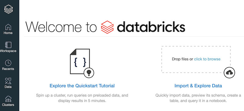
To carry out our operations, Databricks provides a very comfortable working environment based on Notebook (very similar to the one you can use with Anaconda and Jupyter Notebook, or Google Colab, Amazon Sagemaker and several other environments …).
The first thing we have to do is to “link” our Notebook to the Cluster.
Let’s start by importing our dataset in .csv format, after having properly loaded it on the cluster datastore:
file_location = "/FileStore/tables/ais-4.csv"
df = spark.read.format("csv").option("inferSchema",
True).option("header", True).load(file_location)
Let’s visualize its scheme:
df.printSchema()
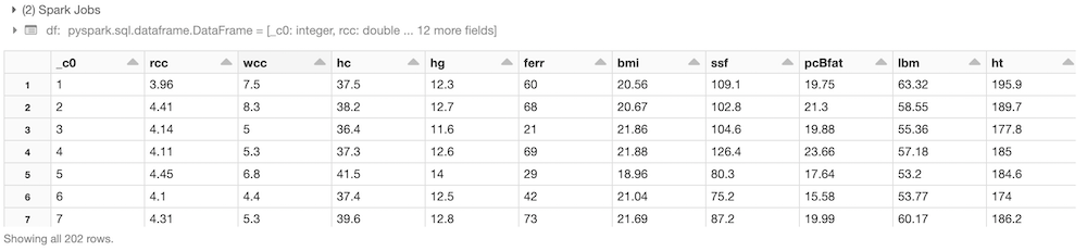
(1) Spark Jobsdf:pyspark.sql.dataframe.DataFrame = [_c0: integer, rcc: double … 12 more fields]root |– _c0: integer (nullable = true) |– rcc: double (nullable = true) |– wcc: double (nullable = true) |– hc: double (nullable = true) |– hg: double (nullable = true) |– ferr: integer (nullable = true) |– bmi: double (nullable = true) |– ssf: double (nullable = true) |– pcBfat: double (nullable = true) |– lbm: double (nullable = true) |– ht: double (nullable = true) |– wt: double (nullable = true) |– sex: string (nullable = true) |– sport: string (nullable = true)
This is the dataset of the Australian athletes blood test parameters, which we have already used in one of our previous linear regression example!
Let’s convert the dataset from csv to parquet, in order to work in lazy execution mode, as already illustrated (this will only need to be done the first time we execute the code):
df.write.save('/FileStore/parquet/ais-4',format='parquet')
Let’s load the data in parquet format and take a look at our dataset!df = spark.read.load("/FileStore/parquet/ais-4")
display(df)
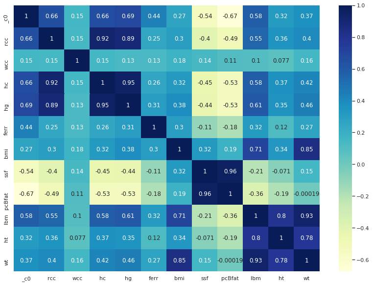
We can now evaluate the feature correlation matrix and perform some proper dimensional reductions:
import matplotlib.pyplot as plt
import seaborn as sns; sns.set()
df2 = df.toPandas()
fig, ax = plt.subplots(figsize=(14,10))
ax = sns.heatmap(df2.corr(), cmap="YlGnBu", annot = True)
df_new=df.drop('rcc','hc','hg','ferr','ssf','pcBfat','sport')
df_new.printSchema()
Let’s split the dataset by male and female:
df_male = df_new.filter(df_new.sex == "m")
df_female = df_new.filter(df_new.sex == "f")
Next, we are going prepare the environment in order to use the pipelines and the MLib libraries: a very powerful set specifically designed for implementing machine learning models on a distributed environments such as Spark!
from pyspark.ml.feature import VectorAssembler
from pyspark.ml.regression import LinearRegression
from pyspark.ml import Pipeline
MLibs require independent features to be passed as a vector and the target label to be predicted as a scalar value:
#set the independent variable vector (features)
assembler = VectorAssembler(inputCols=['bmi', 'wt'],outputCol="features")
We can use the LinearRegression function made available by the MLib, so to predict the athlete’s lbm value (Lean Body Mass index) function of the bmi and wt independent features:
lr = LinearRegression(featuresCol = 'features', labelCol='lbm')
Let’s split the data for the Training phase (80% of the total amount) and for the Test phase (the remaining 20%):
train_df, test_df = train.randomSplit([0.8, 0.2]) ;to be used in case of no Pipeline commands
train_df, test_df = df_male.randomSplit([0.8, 0.2])
It is time to put together the entire ML life cycle by using the pipeline function: in our case, we have a preprocessing step, identified with the resultant of the assembler variable including the feature engineering we have performed previously and the estimator step , the variable lr which implements the linear regression model:
pipeline = Pipeline(stages=[assembler, lr])
Finally, let’s use the pipeline fit method in order to train the model:lr_model = pipeline.fit(train_df)
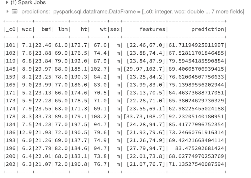
Once the training and validation have been performed, let’s move forward and test the model. To accomplish this step, we’ll invoke the transform method of our pipeline, which we will use to apply the trained model to the test data:
predictions = lr_model.transform(test_df)
predictions.show()
Here is the result of the predictions performed on the test data:
At this point we can use some “Evaluator” functions in order to display the metrics related to the most relevant results of the trained regression model:
from pyspark.ml.evaluation import *
eval_rmse = RegressionEvaluator(labelCol="lbm", predictionCol="prediction", metricName="rmse")
eval_mse = RegressionEvaluator(labelCol="lbm", predictionCol="prediction", metricName="mse")
eval_mae = RegressionEvaluator(labelCol="lbm", predictionCol="prediction", metricName="mae")
eval_r2 = RegressionEvaluator(labelCol="lbm", predictionCol="prediction", metricName="r2")
print('RMSE:', eval_rmse.evaluate(predictions))
print('MSE:', eval_mse.evaluate(predictions))
print('MAE:', eval_mae.evaluate(predictions))
print('R2:', eval_r2.evaluate(predictions))
RMSE and R2 are the two of the most significant parameters for evaluating the accuracy of our regression model. Here are the results:
(4) Spark Jobs
RMSE: 2.4854195595721813
MSE: 6.177310387103976
MAE: 1.5654423776210198
R2: 0.907450608117363
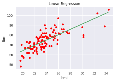
We can also view the regression function trend, in order to get a graphical idea of the result (let’s simplify it by selecting only the bmi independently variable to plot a two-dimensional chart):
import numpy as np
from numpy import polyfit
data = df_male
x1 = data.toPandas()['bmi'].values.tolist()
y1 = data.toPandas()['lbm'].values.tolist()
plt.scatter(x1, y1, color='red', s=30)
plt.xlabel('bmi')
plt.ylabel('lbm')
plt.title('Linear Regression')
p1 = polyfit(x1, y1, 1)
plt.plot(x1, np.polyval(p1,x1), 'g-' )
plt.show()
We have just illustrated an example to adopt some pipeline best practices over a distributed environments with Spark, in order to scale our machine learning life cycle.
There are additional tools coming out on the market to perform pipeline assessment and manage MLOps according to a professional way, thus to improve the governance and scalability… Therefore stay tuned!
Interested in learning more about Machine Learning and AI applications?
Here you can find a book about it:
https://www.amazon.com/dp/B08GFL6NVM